
This article explores the fundamental concepts of database systems, from simple file-based storage to complex distributed architectures. We'll cover the core data structures, algorithms, and design principles that power modern databases, with practical examples and visualizations.
Who Should Read This
Every software engineer who interacts with databases should understand how they work under the hood. Whether you're using MySQL, PostgreSQL, MongoDB, or Cassandra, knowing the underlying principles will help you make better design decisions, troubleshoot performance issues, and understand architectural trade-offs. This article takes you from simple storage concepts to sophisticated distributed systems patterns, giving you the mental models needed to work effectively with any database technology.
Why Do We Need Databases?
Let's start with the simplest possible "database" - a bash script that appends data to a file:
#!/bin/bash

db_set() {
  echo "$1,$2" >> database.txt
}

db_get() {
  grep "^$1," database.txt | sed -e "s/^$1,//" | tail -n 1
}
You can use it like this:
$ db_set 42 '{"name": "Alice", "age": 25}'
$ db_set 43 '{"name": "Bob", "age": 30}'
$ db_get 42
{"name": "Alice", "age": 25}
This tiny "database" actually works! But what's wrong with it? Let's examine its limitations:
Performance Problems
-
Read Performance: The
db_getfunction scans the entire file usinggrep, making itO(n)where n is the total number of records. As your data grows, reads become painfully slow. -
Write Performance: Each write appends to the file, which works fine initially but leads to unbounded file growth, including duplicate keys.
Reliability Issues
-
Durability: The
echocommand writes to the file, but it doesn't guarantee that data has been flushed to stable storage. If your machine crashes, recent writes might be lost. -
Atomicity: If the system crashes during the
echooperation, you might end up with partially written data. -
Isolation: If multiple processes call
db_setordb_getconcurrently, they might interfere with each other, causing race conditions.
Basic Improvements
Let's make some simple improvements:
#!/bin/bash

db_set() {
  # Use flock for isolation
  (
    flock -x 200
    echo "$1,$2" >> database.txt
    # Use fsync for durability
    sync -d database.txt
  ) 200>database.lock
}

db_get() {
  # Use shared lock for reads
  (
    flock -s 200
    grep "^$1," database.txt | sed -e "s/^$1,//" | tail -n 1
  ) 200>database.lock
}
We've addressed some issues:
- Added file locking for isolation
- Added syncing for durability (but partial/corrupt writes are still possible if a crash happens during the write operation)
But we still have fundamental problems:
- The
O(n)read performance - Unbounded file growth with duplicate keys
- No efficient way to update or delete records
These limitations are exactly why we need real database systems with efficient data structures and algorithms.
Buffer Management and Memory Caching
Reading from disk is slow, so databases maintain an in-memory cache of frequently accessed pages, often called the buffer pool.
Buffer pool architecture showing page table mapping disk pages to memory frames
Source: Intel, "Optimizing Write Ahead Logging with Intel Optane Persistent Memory"
The buffer pool manages:
- Page Table: Maps page IDs to their locations in memory
- Replacement Policy: Decides which pages to evict when memory is full (LRU, Clock, etc.)
- Dirty Page Tracking: Identifies pages that have been modified and need to be written back to disk
Optimizing Buffer Management
- Prefetching: When accessing sequential pages, proactively load the next pages
- Scan Sharing: Multiple queries can share scanned pages
- Buffer Pool Bypass: For one-time large scans, avoid polluting the buffer pool
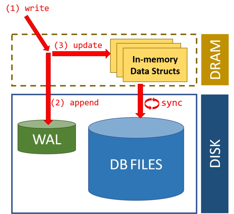
Write-Ahead Logging (WAL)
Before we modify pages in memory, we need a way to ensure durability and atomicity in case of crashes. Write-Ahead Logging (WAL) is a technique used by databases to achieve this.
The key principle of WAL is: Before modifying any data on disk, first record the changes in a log.
Benefits of WAL:
- Atomicity: If a transaction is interrupted, we can roll back using the log
- Durability: Once a transaction commits, its changes are in the log even if the data pages haven't been written to disk
- Performance: We can batch data page writes while ensuring durability through the log
During crash recovery, the database processes the WAL in three phases:
- Analysis: Determine which transactions were active at crash time
- Redo: Replay all changes for committed transactions
- Undo: Roll back changes for uncommitted transactions
Storage Engines: The Heart of Database Systems
A storage engine is responsible for organizing data on disk. The two main families of storage engines are:
- Page-oriented storage engines (e.g., B-Trees used in PostgreSQL, MySQL, Oracle)
- Log-structured storage engines (e.g., LSM-Trees used in LevelDB, RocksDB, Cassandra)
Let's explore both approaches.
B-Tree: The Workhorse of Relational Databases
B-Trees have been the dominant storage engine in databases since the 1970s. Unlike binary trees, B-Trees are specifically optimized for systems that read and write large blocks of data.
How B-Trees Work
A B-Tree is a self-balancing tree data structure that:
- Keeps data sorted
- Allows searches, sequential access, insertions, and deletions in logarithmic time
- Is optimized for systems that read and write large blocks of data
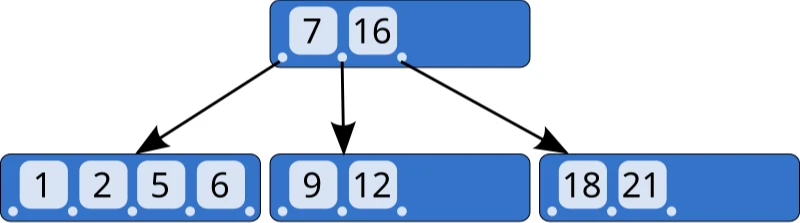
B-Tree Nodes and Disk Blocks Relationship
A critical concept in understanding B-Trees is how they map to physical storage:
-
B-Tree Nodes vs. Disk Blocks:
- A B-Tree node is a logical structure in the tree
- Each node typically maps to one disk block/page (or sometimes multiple)
- Disk blocks are the physical units of I/O (typically 4KB, 8KB, or 16KB)
-
Optimizing for Block Devices:
- B-Trees are designed to minimize disk I/O operations
- Node size is chosen to match disk block size
- This maximizes the fanout (number of children per node)
- Each disk read retrieves a complete node
-
Branching Factor:
- The branching factor (maximum number of children per node) is directly related to disk block size
- Larger blocks = more keys per node = higher branching factor = shorter tree
- For a 16KB page that can store 100 keys, a 3-level B-Tree can index about 1 million records (100³)
B-Tree vs B+ Tree: Key Differences
While B-Trees are widely used, B+ Trees offer important optimizations for database systems:
| Feature | B-Tree | B+ Tree |
|---|---|---|
| Data Storage | Data can be stored in both internal and leaf nodes | Data is stored only in leaf nodes; internal nodes contain only keys |
| Leaf Nodes | Not linked to each other | All leaf nodes are linked in a sequential linked list |
| Node Structure | Each node contains keys and data or keys and pointers | Internal nodes: keys and pointers only Leaf nodes: keys and data |
| Space Efficiency | Less efficient as data is stored throughout the tree | More efficient as internal nodes only store keys |
| Range Queries | Less efficient, may require traversing back up the tree | Very efficient due to linked leaf nodes |
| Height | Potentially shorter for the same data | May be slightly taller |
B+ Trees are preferred in most database systems because:
- They provide better scanning performance (all records are in leaf nodes linked together)
- They have better space utilization in internal nodes (more branching factor)
- They offer more consistent performance (all data is at the same level)
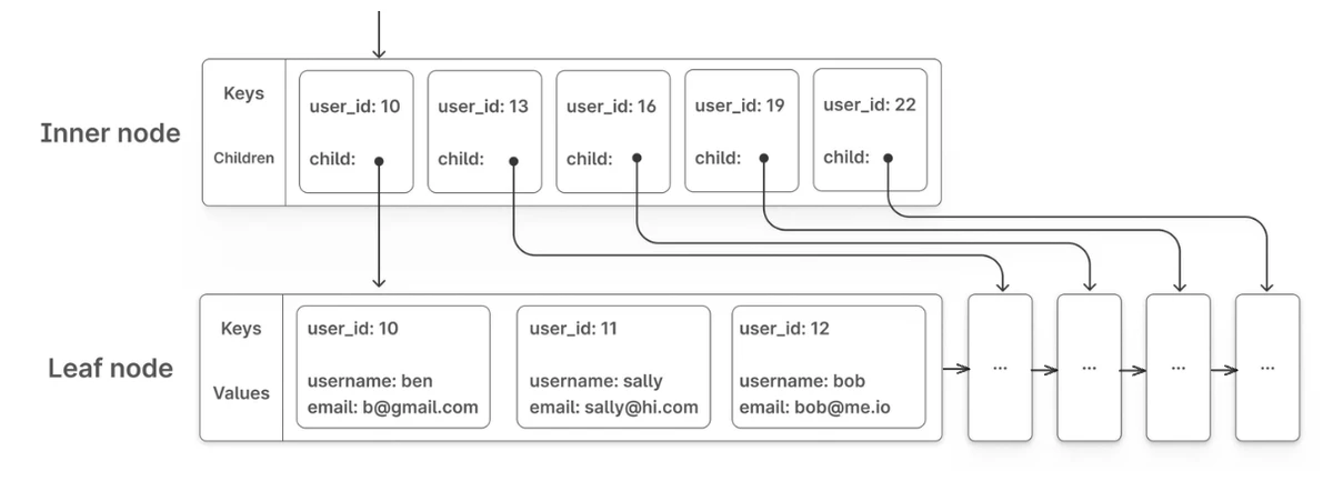
B+ Tree structure showing inner nodes with keys/pointers and leaf nodes with actual data
Source: PlanetScale Blog, "B-trees and database indexes" (https://planetscale.com/blog/btrees-and-database-indexes)
While B+ Trees excel in many scenarios, they have specific strengths and weaknesses for write-heavy workloads:
Pros:
- Predictable Performance: Operations have guaranteed O(log n) time complexity
- Read Optimization: Excellent for workloads that mix reads with writes
- Range Queries: Efficient for range scans even under write load
- In-Place Updates: Ability to update records without creating entirely new structures
- Mature Implementation: Well-understood algorithms with decades of optimization
Cons:
- Random I/O: Each write typically requires multiple random I/O operations
- Write Amplification: Small updates can cause cascade of page splits and merges
- Fragmentation: Over time, pages may become partially empty, wasting space
- Locking Overhead: Traditional B+ Tree implementations often require locking for concurrent updates
- Write Bottlenecks: All writes must update the tree structure, creating potential bottlenecks
For applications with extremely high write volumes, especially those with sequential inserts or time-series data, alternative structures like LSM Trees may provide better performance characteristics.
LSM Trees: Optimizing for Write-Heavy Workloads
Log-Structured Merge Trees (LSM Trees) take a different approach, optimizing for write performance at some cost to reads.
LSM Tree Architecture
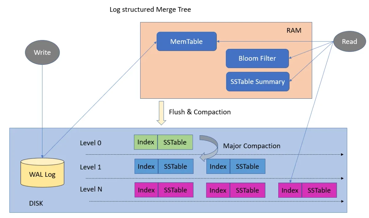
LSM Tree architecture showing MemTable, WAL, and SSTables
Source: Medium, "LSM Trees: The Go-To Data Structure for Databases, Search Engines, and More" (https://medium.com/@dwivedi.ankit21/lsm-trees-the-go-to-data-structure-for-databases-search-engines-and-more-c3a48fa469d2)
LSM Trees have two main components:
- MemTable: An in-memory sorted data structure (often a balanced tree or skiplist)
- SSTable (Sorted String Table): Immutable sorted files on disk
// LSMTree represents the complete storage engine
type LSMTree struct {
	MemTable     *MemTable        // In-memory buffer for recent writes
	WAL          *WAL             // Write-ahead log for durability
	SSTables     []*SSTable       // Sorted immutable files on disk
	Threshold    int              // Size threshold for MemTable flushes
	CompactionMu sync.Mutex       // Lock for compaction operations
}

// MemTable is an in-memory sorted structure for recent writes
type MemTable struct {
	data  map[string][]byte // Using a map for simplicity; skiplist in production
	size  int               // Current size in bytes
}

// SSTable represents an immutable sorted file on disk
type SSTable struct {
	ID          int              // Unique identifier
	FilePath    string           // Path to the file on disk
	BloomFilter *BloomFilter     // Quick membership tests
	Index       *SparseIndex     // Helps locate keys efficiently
}
Write Path: How Data Gets Stored
The write path in an LSM Tree follows these steps:
- Log the write to the WAL for crash recovery
- Add the key-value pair to the in-memory MemTable
- When the MemTable gets full, flush it to disk as an SSTable
- Periodically compact SSTables to manage space
Here's a simplified implementation of the write operation:
// Write adds a key-value pair to the LSM Tree
func (lsm *LSMTree) Write(key string, value []byte) error {
	// 1. First write to WAL for durability
	if err := lsm.WAL.Append(key, value); err != nil {
		return fmt.Errorf("failed to write to WAL: %w", err)
	}

	// 2. Then add to memtable
	lsm.MemTable.Put(key, value)

	// 3. If memtable exceeds threshold, flush to disk
	if lsm.MemTable.Size() >= lsm.Threshold {
		if err := lsm.FlushMemTable(); err != nil {
			return fmt.Errorf("failed to flush memtable: %w", err)
		}
	}

	return nil
}

// Append adds a record to the WAL
func (wal *WAL) Append(key string, value []byte) error {
	// Write key-value pair to log with timestamp
	timestamp := time.Now().UnixNano()
	// ... write to log file ...
	return wal.File.Sync() // Ensure durability
}
When the MemTable gets full, we flush it to disk as a new SSTable:
// FlushMemTable creates a new SSTable from the current memtable
func (lsm *LSMTree) FlushMemTable() error {
	// Prevent concurrent flushes
	lsm.CompactionMu.Lock()
	defer lsm.CompactionMu.Unlock()

	// Convert MemTable to SSTable and write to disk
	sstID := len(lsm.SSTables) + 1
	sstable, err := lsm.createSSTableFromMemTable(sstID)
	if err != nil {
		return err
	}

	// Add to SSTables list (newest first)
	lsm.SSTables = append([]*SSTable{sstable}, lsm.SSTables...)

	// Create new empty MemTable
	lsm.MemTable = NewMemTable()

	// Maybe trigger compaction in background
	if len(lsm.SSTables) > 10 {
		go lsm.Compact()
	}

	return nil
}
Read Path: How Data Is Retrieved
Reading from an LSM Tree involves checking multiple locations:
- First check the MemTable (most recent writes)
- Then check SSTables from newest to oldest
- Use optimization techniques to avoid unnecessary disk reads
Here's how a read operation works:
// Read retrieves a value for the given key
func (lsm *LSMTree) Read(key string) ([]byte, bool) {
	// 1. First check memtable (most recent writes)
	if value, found := lsm.MemTable.Get(key); found {
		return value, true
	}

	// 2. Then check SSTables, from newest to oldest
	for _, sstable := range lsm.SSTables {
		// Optimization: Use bloom filter to skip tables that definitely don't have the key
		if !sstable.BloomFilter.MightContain(key) {
			continue // Key definitely not in this SSTable
		}

		// Use sparse index to efficiently locate the key
		if value, found := sstable.Get(key); found {
			return value, true
		}
	}

	// Key not found anywhere
	return nil, false
}
Optimization: Bloom Filters
A Bloom filter is a space-efficient probabilistic data structure that tells you if an element is definitely not in a set or might be in a set.
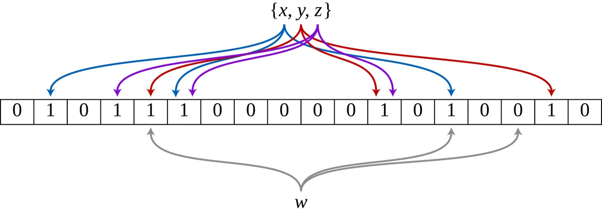
Bloom filter data structure showing set membership testing with hash functions
Source: Wikipedia, "Bloom filter" (https://en.wikipedia.org/wiki/Bloom_filter)
In the illustration above, we see how a Bloom filter works in practice:
- Adding elements: When keys
x,y, andzare added to the filter, each key is hashed using multiple hash functions. - Setting bits: The hash results determine which positions in the bit array to set to
1. - Membership test: To check if key
wexists, we hash it with the same functions and check if all corresponding bits are1. - False positives: If all bits are
1(like for keywin the diagram), the element might be in the set - this could be a false positive. - Definite negatives: If any bit is
0, the element is definitely not in the set (no false negatives).
This property makes Bloom filters perfect for LSM Trees - we can quickly skip SSTables that definitely don't contain a key, avoiding expensive disk reads.
For each SSTable, we maintain a Bloom filter to avoid unnecessary disk reads:
// BloomFilter provides probabilistic set membership tests
type BloomFilter struct {
	Bits    []bool               // Bit array
	HashFns []func(string) int   // Hash functions
}

// MightContain returns false if definitely not in set, true if might be in set
func (bf *BloomFilter) MightContain(key string) bool {
	for _, hashFn := range bf.HashFns {
		position := hashFn(key)
		if !bf.Bits[position] {
			return false // Definitely not in the set
		}
	}
	return true // Might be in the set
}

// Add adds an element to the Bloom filter
func (bf *BloomFilter) Add(key string) {
	for _, hashFn := range bf.HashFns {
		position := hashFn(key)
		bf.Bits[position] = true
	}
}
Optimization: Sparse Indices
Sparse indices optimize disk access by storing the positions of only a subset of keys:
// SparseIndex helps locate keys within an SSTable
type SparseIndex struct {
	Offsets    map[string]int64  // Sample key -> file offset
	SampleRate int               // Sample every Nth key
}

// FindBlock returns the file offset to start searching from
func (si *SparseIndex) FindBlock(key string) int64 {
	// Find the largest sampled key <= target key
	var bestKey string
	var bestOffset int64

	for sampledKey, offset := range si.Offsets {
		if sampledKey <= key && (bestKey == "" || sampledKey > bestKey) {
			bestKey = sampledKey
			bestOffset = offset
		}
	}

	if bestKey == "" {
		return 0 // Start from beginning
	}

	return bestOffset
}
When looking for a key in an SSTable:
- Use the sparse index to find the closest indexed key ≤ the target
- Start reading from that position
- Scan forward until finding the key or confirming it's not there
This dramatically reduces the amount of data we need to scan through.
SSTable Format and Searching
When we search within an SSTable, we use both the Bloom filter and sparse index:
// Get retrieves a value from an SSTable
func (sst *SSTable) Get(key string) ([]byte, bool) {
	// 1. Use sparse index to find where to start reading
	offset := sst.Index.FindBlock(key)

	// 2. Open file and seek to that position
	file, err := os.Open(sst.FilePath)
	if err != nil {
		return nil, false
	}
	defer file.Close()

	file.Seek(offset, io.SeekStart)

	// 3. Scan entries until we find the key or pass where it would be
	for {
		// Read key and value
		keyLen, valueLen, err := readLengths(file)
		if err != nil {
			return nil, false
		}

		entryKey, err := readKey(file, keyLen)
		if err != nil {
			return nil, false
		}

		// Found the key?
		if entryKey == key {
			value, err := readValue(file, valueLen)
			return value, err == nil
		}

		// Gone past where the key would be?
		if entryKey > key {
			return nil, false
		}

		// Skip this value and continue
		file.Seek(int64(valueLen), io.SeekCurrent)
	}
}
Compaction: Managing SSTables
Over time, many SSTables accumulate. Compaction merges them to:
- Reclaim space from deleted/overwritten entries
- Reduce the number of files to check during reads
- Improve read performance
// Compact merges SSTables to optimize storage and performance
func (lsm *LSMTree) Compact() error {
	lsm.CompactionMu.Lock()
	defer lsm.CompactionMu.Unlock()

	// Select SSTables to compact (simplistic approach)
	if len(lsm.SSTables) < 2 {
		return nil
	}

	// Merge two oldest SSTables
	oldestIdx := len(lsm.SSTables) - 2
	merged, err := lsm.mergeSSTables(
		lsm.SSTables[oldestIdx],
		lsm.SSTables[oldestIdx+1],
	)

	if err != nil {
		return err
	}

	// Replace the old SSTables with the merged one
	lsm.SSTables = append(
		lsm.SSTables[:oldestIdx],
		append([]*SSTable{merged}, lsm.SSTables[oldestIdx+2:]...)...,
	)

	// Clean up old files
	// ...

	return nil
}
LSM Trees vs B-Trees
| Aspect | LSM Trees | B-Trees |
|---|---|---|
| Write Performance | • Better for high-volume writes | • Random I/O for each write |
| Read Performance | • Must check multiple files (MemTable + SSTables) | • Direct path to data via tree traversal |
| Maintenance | • Background compaction required | • No background compaction needed |
| Space Efficiency | • Better overall due to compaction | • Pages may become partially empty |
| Crash Recovery | • WAL (Write-Ahead Log) for durability | • WAL or journaling required |
| Ideal Use Cases | • Write-heavy workloads | • Read-heavy workloads |
Transaction Processing and Isolation Levels
A transaction is a sequence of operations that is treated as a single logical unit of work, which should maintain the ACID properties:
- Atomicity: All operations complete successfully or none of them do
- Consistency: The database moves from one valid state to another
- Isolation: Concurrent transactions don't interfere with each other
- Durability: Once committed, changes persist even in case of failures
Concurrency Problems
When multiple transactions run concurrently, several anomalies can occur:
1. Dirty Reads
A dirty read occurs when one transaction reads data that has been modified but not yet committed by another transaction.
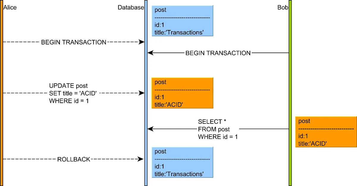
Illustration of a dirty read concurrency anomaly where a transaction reads uncommitted data
Source: "High-Performance Java Persistence" by Vlad Mihalcea
2. Dirty Writes
One transaction overwrites an uncommitted value written by another transaction
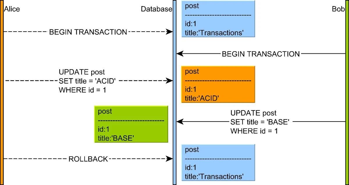
Illustration of a dirty write anomaly where a transaction overwrites uncommitted data from another transaction
Source: "High-Performance Java Persistence" by Vlad Mihalcea
3. Lost Updates
A lost update occurs when two transactions read and then update the same data, with the second transaction "losing" the update of the first one.
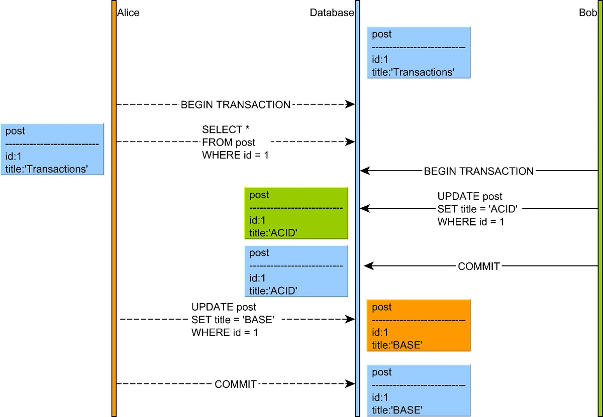
Illustration of a lost update anomaly where two transactions read and update the same data, with one change being lost
Source: "High-Performance Java Persistence" by Vlad Mihalcea
4. Non-Repeatable Reads
A non-repeatable read occurs when a transaction reads the same row twice and gets different values because another transaction modified and committed the data between reads.
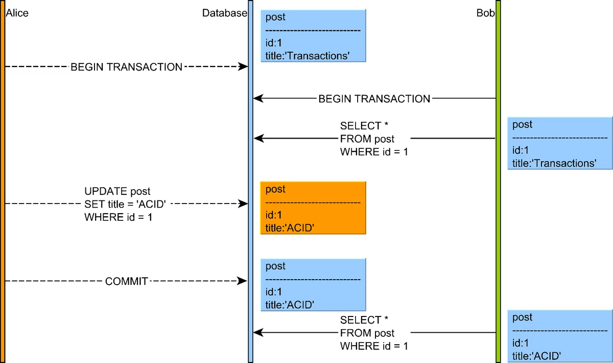
Illustration of a non-repeatable read anomaly where a transaction reads the same row twice but gets different values
Source: "High-Performance Java Persistence" by Vlad Mihalcea
5. Read Skew
Read skew occurs when a transaction reads related data that is updated by another transaction, causing a skewed view that violates data constraints.
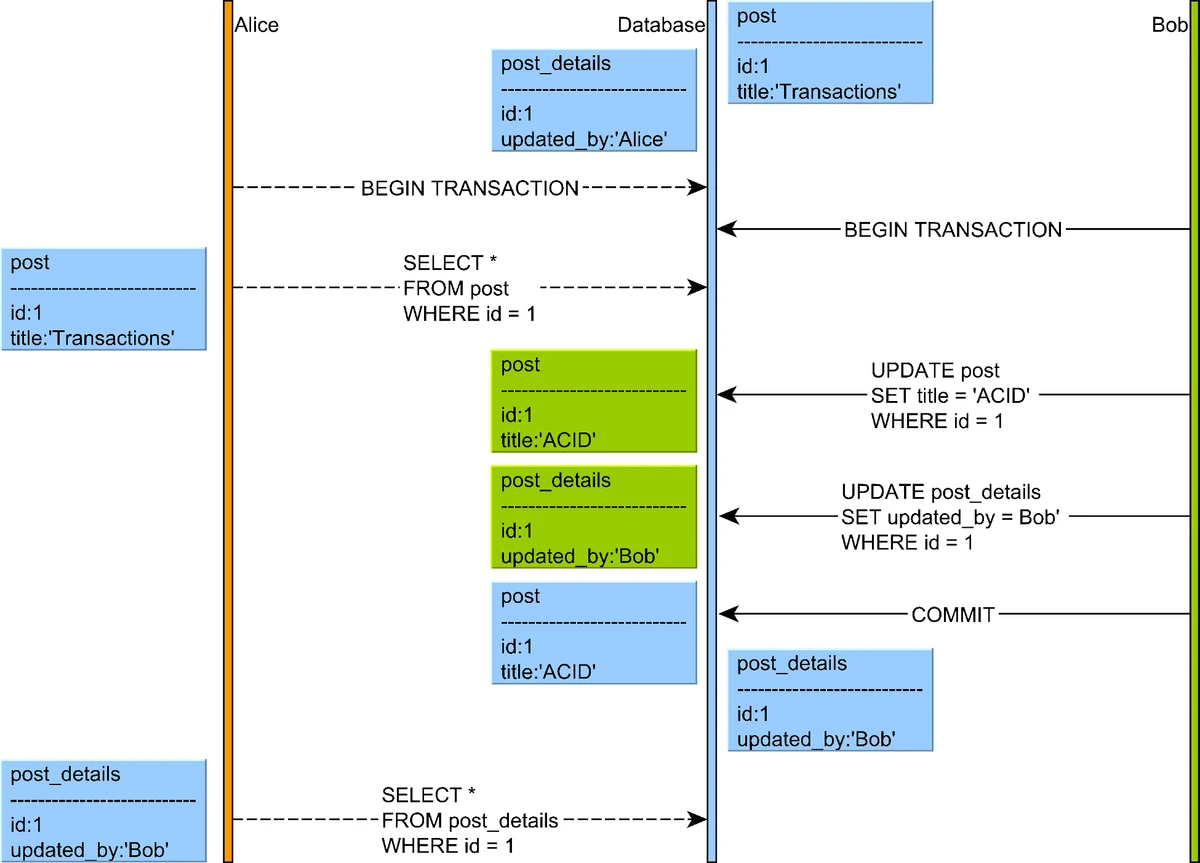
Illustration of a read skew anomaly where a transaction reads related data that is updated by another transaction
Source: "High-Performance Java Persistence" by Vlad Mihalcea
6. Write Skew
Write skew occurs when two transactions read an overlapping data set, make disjoint updates based on what they read, and jointly create an inconsistent result.
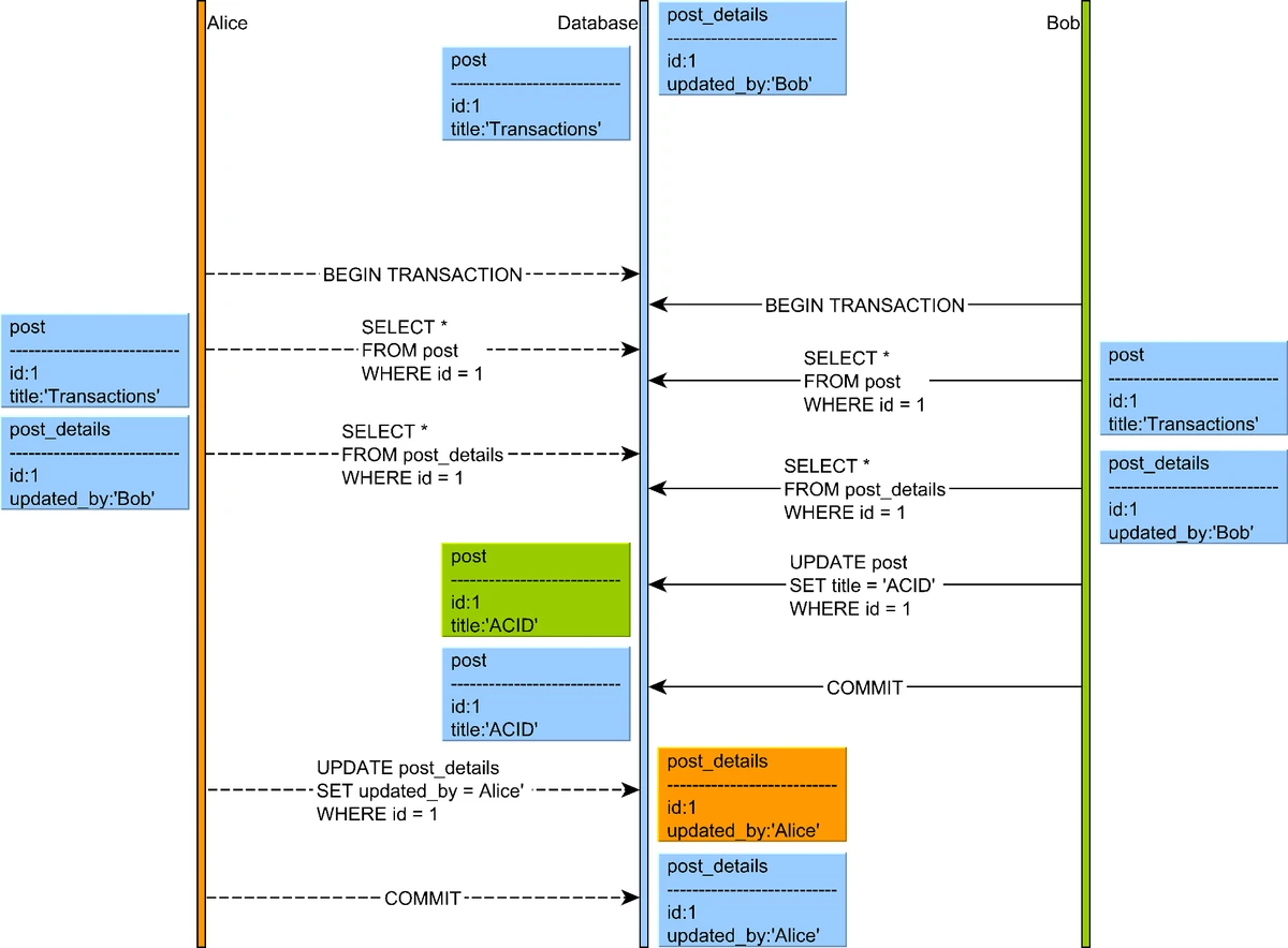
Illustration of a write skew anomaly where two transactions read an overlapping data set and make disjoint updates
Source: "High-Performance Java Persistence" by Vlad Mihalcea
7. Phantom Reads
A phantom read occurs when a transaction executes a query twice, and the second result includes rows that weren't visible in the first result (or vice versa) because another transaction added or removed qualifying rows.
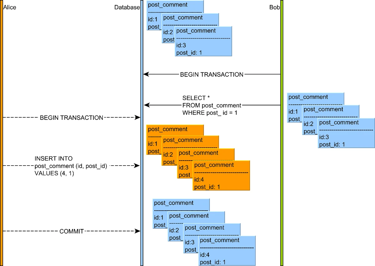
Illustration of a phantom read anomaly where a transaction sees rows that weren't visible in a previous read
Source: "High-Performance Java Persistence" by Vlad Mihalcea
Isolation Levels and Their Implementation
Databases provide different isolation levels to balance consistency and performance:
| Isolation Level | Lost Updates | Dirty Reads | Non-Repeatable Reads | Read Skew | Write Skew | Phantom Reads |
|---|---|---|---|---|---|---|
| READ UNCOMMITTED | Prevented | Possible | Possible | Possible | Possible | Possible |
| READ COMMITTED | Prevented | Prevented | Possible | Possible | Possible | Possible |
| REPEATABLE READ | Prevented | Prevented | Prevented | Prevented | Possible | Possible |
| SERIALIZABLE | Prevented | Prevented | Prevented | Prevented | Prevented | Prevented |
1. READ UNCOMMITTED
The weakest isolation level, allowing transactions to see uncommitted data from other transactions.
2. READ COMMITTED
Prevents dirty reads by only showing committed data, but allows non-repeatable reads.
Anomalies Prevented:
- Dirty Writes: Exclusive locks on modified rows until transaction commits
- Dirty Reads: Maintains committed and uncommitted versions, with readers seeing only committed data
3. REPEATABLE READ
Prevents both dirty reads and non-repeatable reads by using snapshot isolation.
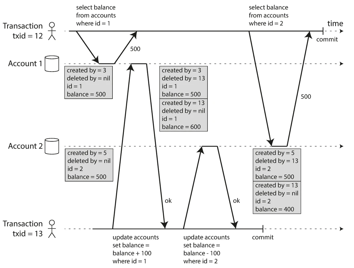
Snapshot isolation implemented with multi-version concurrency control (MVCC)
Source: "Designing Data-Intensive Applications" by Martin Kleppmann (O'Reilly Media, 2017)
Implementation with MVCC (Multi-Version Concurrency Control):
- Each transaction works with a consistent snapshot of the database as of the start time
- Database maintains multiple versions of rows (hence "multi-version")
- Readers never block writers and writers never block readers
- Each version is timestamped or tagged with the transaction ID that created it
- Transactions only see data from transactions that were committed before their start time
- For snapshot isolation, each transaction is assigned a transaction ID (TID)
- When a transaction reads data, it ignores versions created by transactions with higher TIDs
Anomalies Prevented:
- Non-Repeatable Reads: Each transaction operates on a consistent snapshot of the database
4. SERIALIZABLE
The strongest isolation level, preventing all concurrency anomalies.
Implementation Techniques:
-
Two-Phase Locking (2PL):
- Locks are acquired during execution and only released at the end
- Predicate locks or index-range locks prevent phantom reads
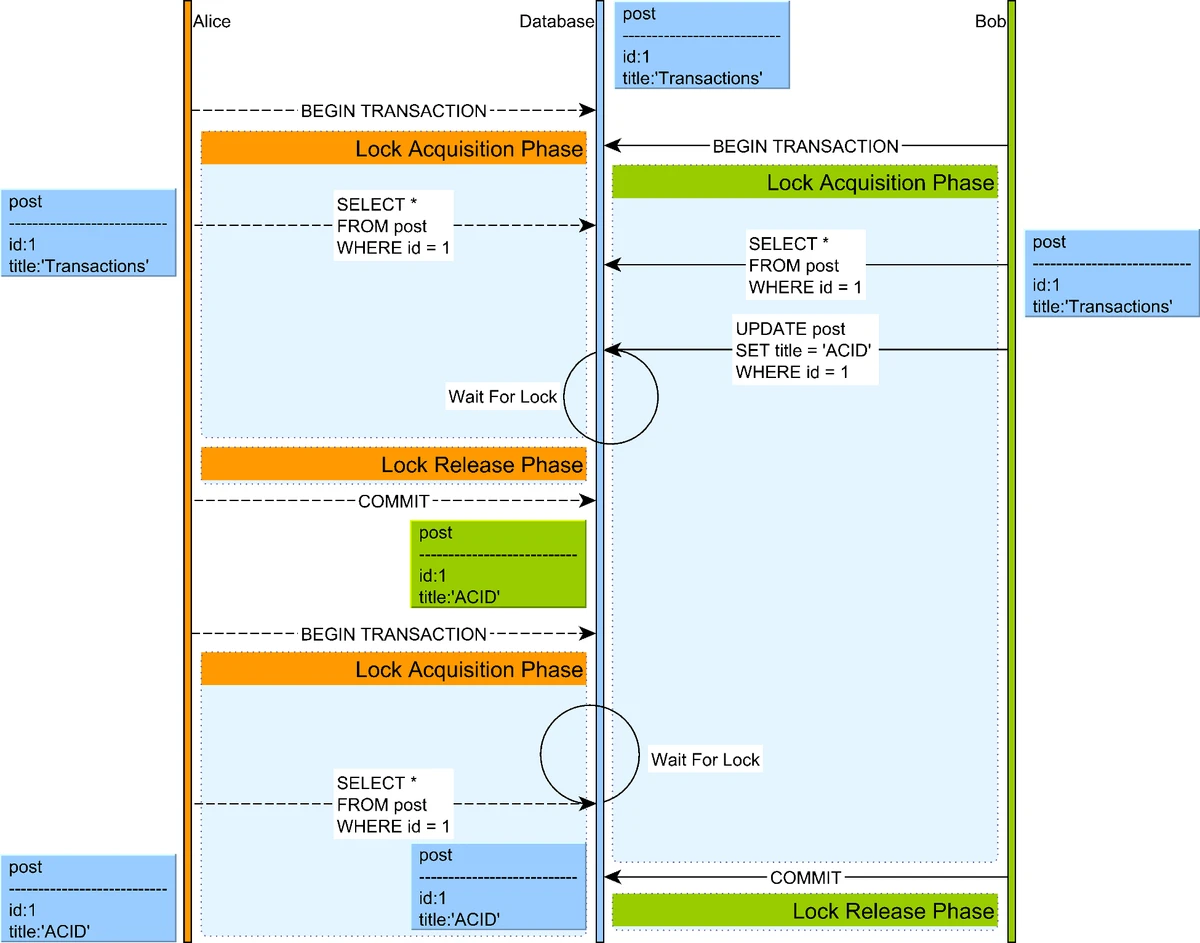
Two-phase locking example
Source: "High-Performance Java Persistence" by Vlad MihalceaDeadlocks in Two-Phase Locking:
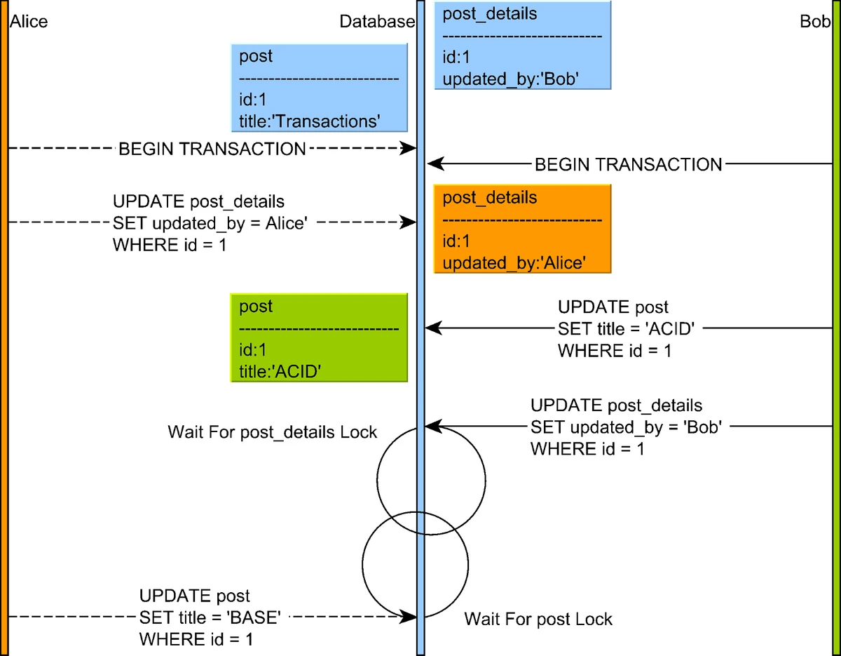
A significant challenge with 2PL is deadlocks, which occur when two or more transactions are waiting for each other to release locks, resulting in a circular dependency. For example, if Transaction A holds a lock on resource X and waits for resource Y, while Transaction B holds a lock on Y and waits for X, neither can proceed.
Deadlock scenario where transactions are waiting for locks held by each other
Source: "High-Performance Java Persistence" by Vlad MihalceaDatabase systems detect deadlocks by maintaining a wait-for graph and checking for cycles. When a deadlock is detected, one of the transactions is chosen as a victim and aborted, allowing others to proceed.
-
Serializable Snapshot Isolation (SSI):
- Tracks dependencies between transactions
- Detects potential serialization anomalies and aborts affected transactions
-
Serial Execution:
- Simply run one transaction at a time
- Only practical for in-memory databases with very fast transactions
Anomalies Prevented: All anomalies (dirty reads, dirty writes, non-repeatable reads, phantom reads, lost updates, read skew, write skew)
Practical Considerations in Isolation Level Selection
When choosing isolation levels for your application, consider:
-
Performance vs. Correctness Trade-offs:
- Weaker isolation levels generally offer better performance but fewer guarantees
- Stronger isolation levels may cause more blocking or aborts
-
Application-Specific Requirements:
- Some applications can tolerate certain anomalies but not others
- Consider what guarantees your business logic needs
-
Transaction Length:
- Keep transactions as short as possible, especially at higher isolation levels
- Long-running transactions at SERIALIZABLE isolation can severely impact concurrency
Most applications use READ COMMITTED as a reasonable default, upgrading specific transactions that require stronger guarantees.
Handling Lost Updates
Lost updates occur when two transactions read and then update the same data concurrently. There are two main approaches to handle them:
| Approach | Pros | Cons |
|---|---|---|
| Pessimistic Locking | • Never needs to abort transactions | • Lower concurrency |
| Optimistic Concurrency Control | • Higher concurrency for read-heavy workloads | • Transactions might need to be retried |
Pessimistic Locking Example
func updateWithPessimisticLock(txn *Transaction, accountID int, amount int) error {
    // Acquire exclusive lock BEFORE reading
    if !lockManager.AcquireExclusiveLock(txn, fmt.Sprintf("account:%d", accountID)) {
        return ErrLockTimeout
    }
    defer lockManager.ReleaseExclusiveLock(txn, fmt.Sprintf("account:%d", accountID))

    // Now safe to read and update
    account := db.GetAccount(accountID)
    account.Balance += amount
    db.UpdateAccount(account)

    return nil
}
Optimistic Concurrency Control Example
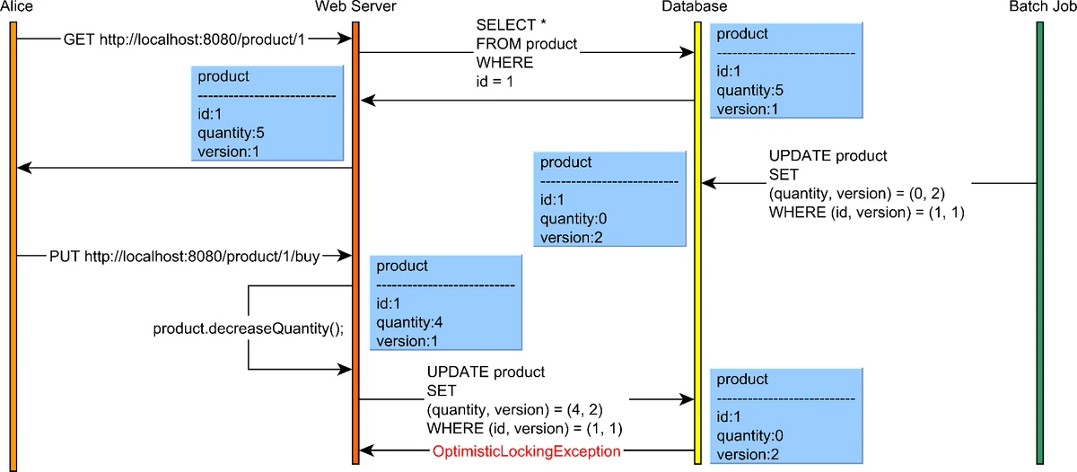
Optimistic locking workflow showing version checking during concurrent updates
Source: "High-Performance Java Persistence" by Vlad Mihalcea
func updateWithOptimisticCC(txn *Transaction, accountID int, amount int) error {
    // Read and remember the version
    account := db.GetAccount(accountID)
    initialVersion := account.Version

    // Modify locally
    account.Balance += amount

    // Try to commit changes - only succeeds if version hasn't changed
    if !db.CompareAndSwap(accountID, initialVersion, account) {
        // Someone else modified the account - conflict!
        return ErrConcurrentModification
    }

    return nil
}
Specialized Storage Models
Beyond row-based and document storage, specialized storage models optimize for particular query patterns and use cases.
Inverted Indexes: Powering Full-Text Search
Inverted indexes are the core data structure behind search engines like Elasticsearch. They map terms to the documents that contain them, enabling efficient full-text search.
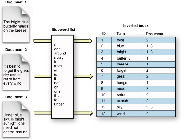
Inverted index structure showing how words map to document references
Source: GitHub repository "Inverted-index-python" by Noureldin2303 (https://github.com/Noureldin2303/Inverted-index-python)
How Inverted Indexes Work
An inverted index reverses the relationship between documents and terms - instead of mapping documents to the words they contain, it maps words to the documents that contain them. This makes searching for documents by keywords extremely efficient.
Key components:
- Dictionary: A sorted list of all unique terms in the corpus
- Posting lists: For each term, a list of document IDs containing that term
- Term frequency information: How often each term appears in each document
- Position information: Where in the document each term appears
For example, with documents:
- Doc1: "The quick brown fox"
- Doc2: "Quick brown foxes leap"
- Doc3: "Lazy dogs sleep"
The inverted index would look like:
brown  -> [Doc1, Doc2]
dogs   -> [Doc3]
fox    -> [Doc1]
foxes  -> [Doc2]
lazy   -> [Doc3]
leap   -> [Doc2]
quick  -> [Doc1, Doc2]
sleep  -> [Doc3]
the    -> [Doc1]
When a user searches for "quick brown", the search engine:
- Looks up "quick" → [Doc1, Doc2]
- Looks up "brown" → [Doc1, Doc2]
- Intersects these sets → [Doc1, Doc2]
- Ranks these documents based on relevance
This approach makes full-text search operations incredibly fast compared to scanning through documents sequentially.
Column-Oriented Storage
Unlike row-oriented databases where all columns of a row are stored together, column stores group values from the same column together on disk.
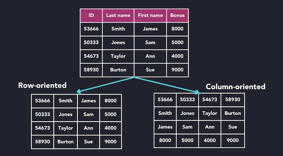
Comparison between row-oriented and column-oriented database storage models
Source: QuestDB, "What Is a Columnar Database?" (https://questdb.com/glossary/columnar-database/)
Key Characteristics
Advantages:
- Analytical Queries: Efficiently reads specific columns across many rows
- Compression: Better compression ratios (10:1) as column values are often similar
- Vectorized Processing: Column operations can leverage CPU SIMD instructions
Disadvantages:
- Write Performance: Less efficient for frequent small updates
- Row Lookups: Retrieving complete rows requires reading from multiple column files
- Transaction Complexity: More challenging to implement ACID transactions
Example: To find the average employee age:
- Row store: Load all employee records, extract age from each, then calculate
- Column store: Load only the "Ages" column and calculate directly
This difference becomes significant at scale, making column stores ideal for OLAP workloads.
Distributed Databases
As data volumes grow, a single machine becomes insufficient. Distributed databases spread data across multiple machines.
Partitioning (Sharding)
Partitioning divides the data into smaller subsets that can be stored on different nodes.
Hash Partitioning
The simplest approach is to use hash(key) % num_nodes:
function determine_node(key, num_nodes):
    return hash(key) % num_nodes
Problem: When you add or remove nodes, almost all keys need to be redistributed.
Consistent Hashing
Consistent hashing minimizes the number of keys that need to be moved when nodes are added or removed.
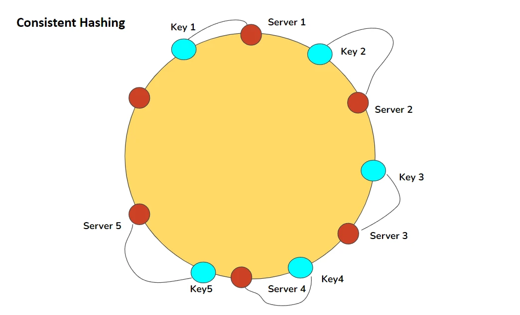
Consistent hashing ring showing key and server distribution
Source: Pratima Upadhyay, "Consistent Hashing" (https://www.linkedin.com/pulse/consistent-hashing-pratima-upadhyay/)
- Map both nodes and keys to positions on a ring
- For each key, go clockwise from the key's position and use the first node encountered
- When a node is added/removed, only keys between that node and its predecessor need to be moved
Implementation: Virtual Nodes
To distribute load more evenly, each physical node can be represented by multiple virtual nodes on the ring:
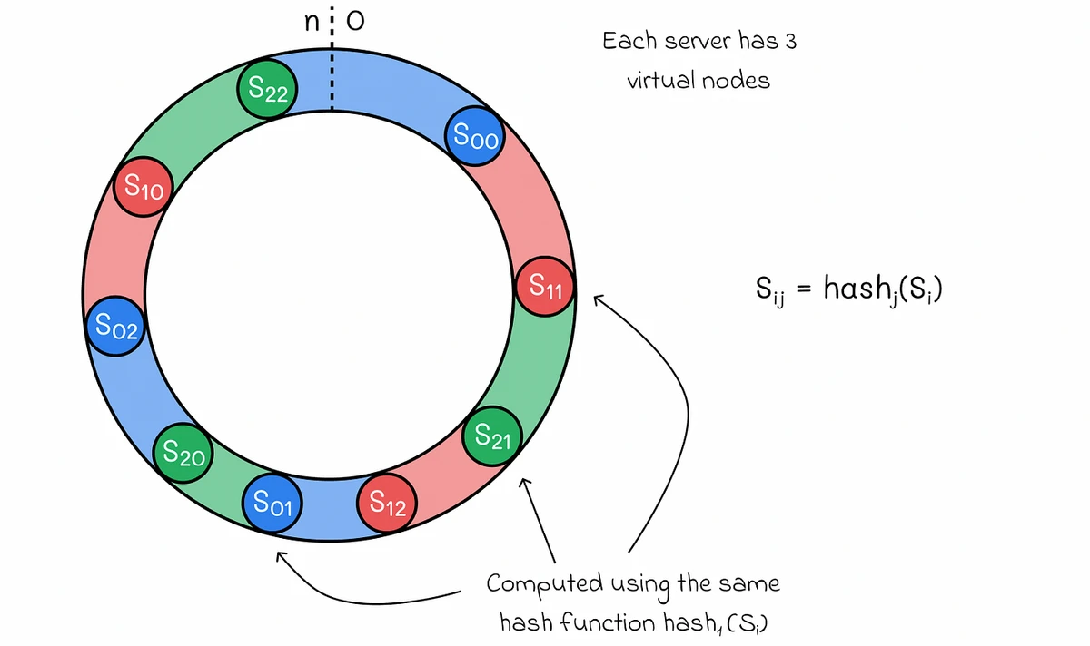
Virtual nodes in consistent hashing for better load distribution
Source: Medium, "System Design: Consistent Hashing" (https://medium.com/data-science/system-design-consistent-hashing-43ddf48d2d32)
Replication
Replication stores copies of the same data on multiple nodes for fault tolerance and read scalability.
Single-Leader Replication
One node is designated as the leader, handling all writes. Writes are propagated to follower nodes.
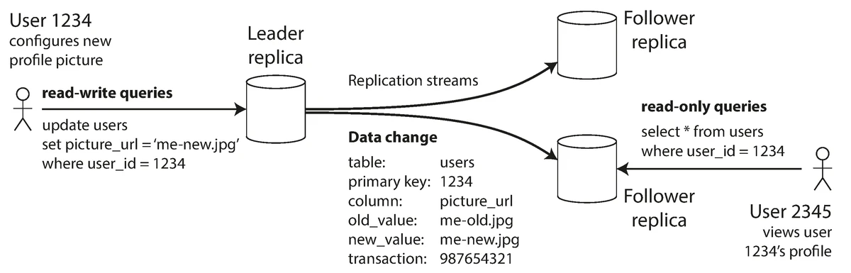
Single-leader replication model showing write path through leader to followers
Source: "Designing Data-Intensive Applications" by Martin Kleppmann (O'Reilly Media, 2017)
Synchronous Versus Asynchronous Replication:
Synchronous: Leader waits for follower acknowledgment before confirming write.
- Pros: Guarantees up-to-date replicas, no data loss if leader fails
- Cons: Higher write latency, leader blocked if follower is slow/unavailable
Asynchronous: Leader doesn't wait for follower acknowledgment.
- Pros: Better performance, resilient to follower failures
- Cons: Potential data loss if leader fails before replication
Problems with Replication Lag
In asynchronous replication systems, replicas may lag behind the leader, causing several consistency problems for clients:
Reading Your Own Writes
If a user writes data to the leader and then tries to read it from a lagging follower, they might not see their own writes.
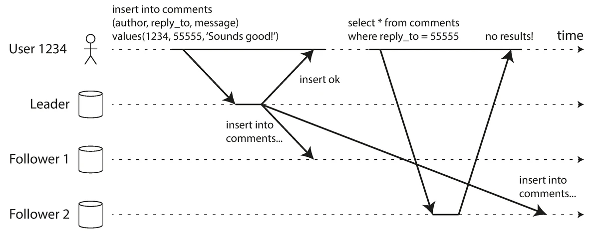
Illustration of the reading-your-own-writes consistency issue in asynchronous replication
Source: "Designing Data-Intensive Applications" by Martin Kleppmann (O'Reilly Media, 2017)
Solution: Read-After-Write Consistency:
- Read from the leader
Monotonic Reads
A user might see data appear and then disappear if they read from different replicas that have different lag.
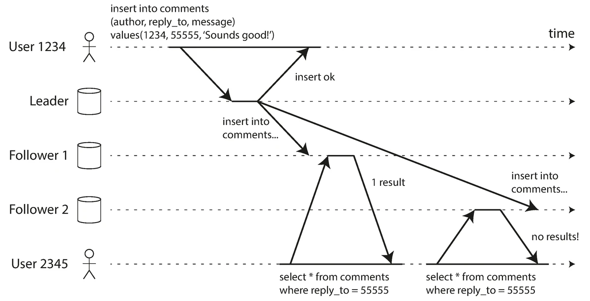
Illustration of the monotonic reads consistency issue with different replicas
Source: "Designing Data-Intensive Applications" by Martin Kleppmann (O'Reilly Media, 2017)
Solution:
- Ensure each user always reads from the same replica
- Session or user-based routing to a specific replica
- Routing based on a consistent hash of the user ID
Consistent Prefix Reads
If replicas process writes in different orders, a reader might see events out of order.
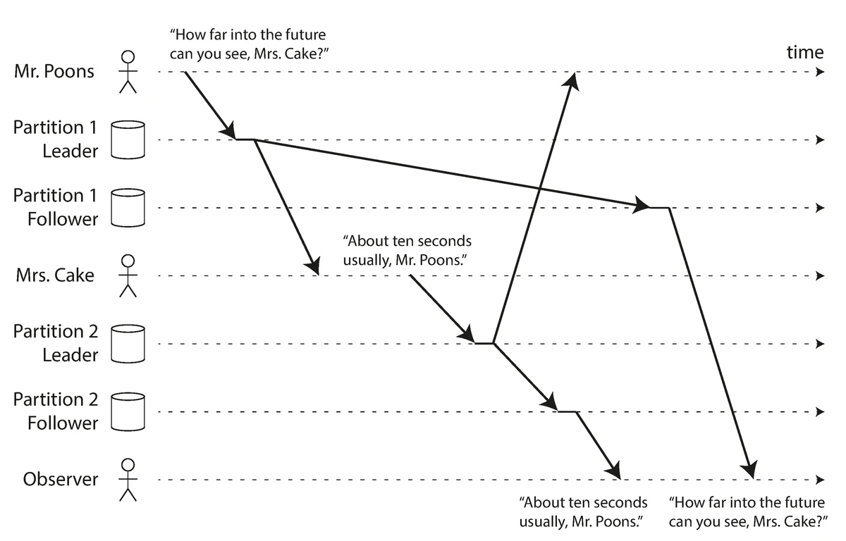
Illustration of the consistent prefix reads problem with out-of-order processing
Source: "Designing Data-Intensive Applications" by Martin Kleppmann (O'Reilly Media, 2017)
Solution:
- Causally related writes should be written to the same partition
- Use sequence numbers or timestamps to order writes
- Track and enforce causal dependencies between operations
Implementation of Replication Logs
Several methods are used to implement leader-based replication:
| Replication Method | Description | Pros | Cons |
|---|---|---|---|
| Statement-Based Replication | The leader logs SQL statements and sends them to followers to execute. Example: UPDATE users SET name = 'John' WHERE id = 123; | • Compact log entries for simple statements | • Non-deterministic functions (NOW(), RAND()) produce different values on replicas |
| Write-Ahead Log (WAL) Shipping | The leader sends its low-level storage engine write-ahead log to followers. Example: XID=12345 UPDATE rel=16385 off=234 len=42 data=... | • Exact reproduction of data structures on followers | • Tightly coupled to storage engine internals |
| Logical (Row-Based) Log Replication | The leader creates a logical log of row-level changes separate from the storage engine. Example: table=users, id=123, column=name, old_value='Jim', new_value='John' | • Works with any SQL statements | • Logs may be larger for wide tables |
| Trigger-Based Replication | Uses database triggers to capture changes and apply them to different systems. Example: CREATE TRIGGER replicate_trigger AFTER INSERT OR UPDATE ON source_table FOR EACH ROW EXECUTE FUNCTION replicate_to_replica(); | • Flexible filtering and transformation | • Higher overhead than built-in replication |
Multi-Leader Replication
Multiple nodes can accept writes, which are then propagated to other nodes.
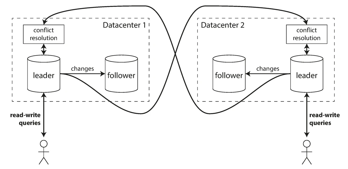
Multi-leader replication model with writes coordinated between multiple leader nodes
Source: "Designing Data-Intensive Applications" by Martin Kleppmann (O'Reilly Media, 2017)
Use Cases for Multi-Leader Replication:
-
Multi-Datacenter Operation:
- Each datacenter has its own leader
- Reduced latency for writes within each datacenter
- Better tolerance of datacenter outages
-
Offline Operation:
- Local "leader" on mobile device or laptop
- Allows operation while disconnected
- Syncs and resolves conflicts upon reconnection
-
Collaborative Editing:
- Each user has a local "leader"
- Changes are propagated asynchronously
- Conflict resolution preserves everyone's changes
Handling Write Conflicts
When multiple leaders accept writes to the same data simultaneously, conflicts can occur:
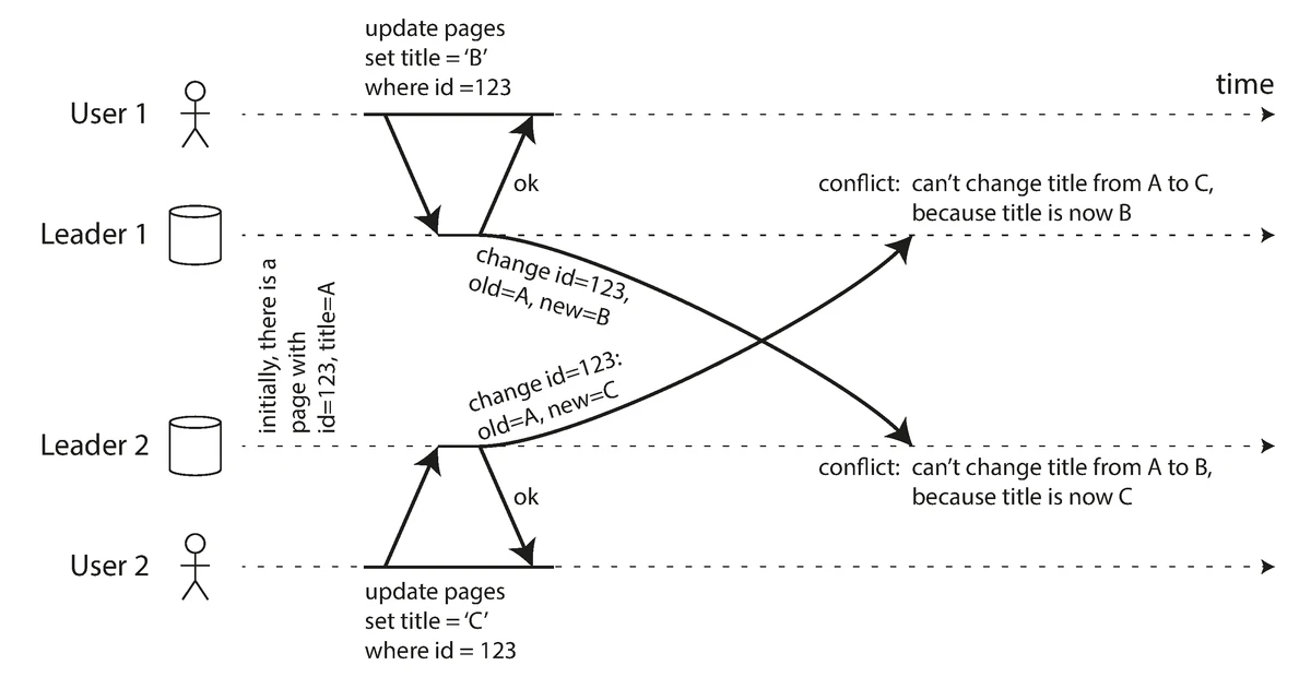
Write conflicts in multi-leader replication when concurrent updates occur on different leaders
Source: "Designing Data-Intensive Applications" by Martin Kleppmann (O'Reilly Media, 2017)
Conflict Resolution Strategies:
-
Last Write Wins (LWW):
- Each write is assigned a timestamp
- The write with the latest timestamp is chosen
- Simple but can lose data
-
Custom Conflict Resolution Logic:
- Application-specific rules based on data semantics
- Example: For a shopping cart, merge the item sets
-
Conflict-Free Replicated Data Types (CRDTs):
- Special data structures designed to be merged automatically
- Example: Counter that can only increment, never decrement
- Ensures eventual consistency without application intervention
-
Explicit User Resolution:
- Present conflicts to users and let them decide
- Stores conflicting versions until resolution
- Used in version control systems like Git
Leaderless Replication
Any node can accept writes; clients coordinate with multiple nodes or any node in the cluster can act as a coordinator. This creates a highly available system without a single point of failure.
Leaderless replication model where clients can write to any node in the cluster
Source: "Designing Data-Intensive Applications" by Martin Kleppmann (O'Reilly Media, 2017)
Quorum Consensus
In leaderless replication systems, we need a way to ensure consistency despite node failures. Quorum consensus provides this guarantee through a simple mathematical rule.
With N replicas, each write must be confirmed by W nodes, and each read must query at least R nodes:
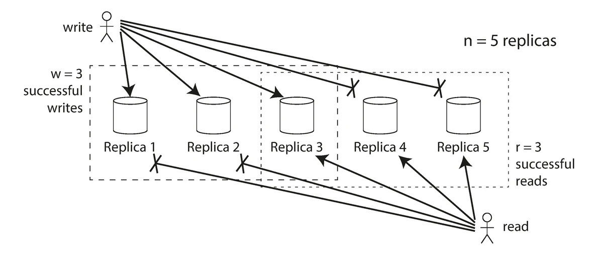
Quorum consensus in leaderless replication to maintain consistency
Source: "Designing Data-Intensive Applications" by Martin Kleppmann (O'Reilly Media, 2017)
When W + R > N, we ensure that there's always at least one node that participates in both the write and read operations, guaranteeing that a read will see the most recent write:
- N = Total number of replicas (typically 3 or 5)
- W = Write quorum (number of nodes that must acknowledge a write)
- R = Read quorum (number of nodes that must respond to a read)
Common configurations:
- W = N, R = 1: Fast reads, but vulnerable to unavailability for writes
- W = 1, R = N: Fast writes, but vulnerable to unavailability for reads
- W = R = (N+1)/2: Balanced approach (e.g., 2 of 3, or 3 of 5)
The trade-off is between availability and consistency: higher values of W and R improve consistency but reduce availability during node failures.
The replication system should ensure that eventually all the data is copied to every replica. After an unavailable node comes back online, how does it catch up on the writes that it missed? Two mechanisms are often used in Dynamo-style datastores:
Read Repair:
- When a client reads from multiple nodes and detects inconsistencies, it writes the newest version back to the outdated replicas
- Works well for frequently read data
- Requires no additional infrastructure
- Passive approach that only fixes data that's actually being read
Anti-Entropy Process:
- Background process that continuously looks for differences between replicas
- Copies missing data from one replica to another
- Doesn't operate in any particular order (unlike leader-based replication logs)
- Ensures all data is eventually consistent, even if rarely accessed
- May have significant delays before convergence
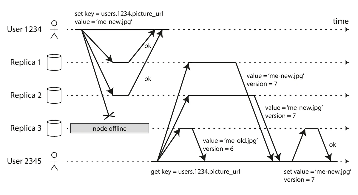
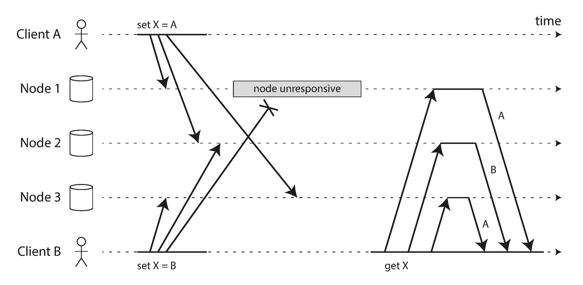
Concurrent Writes and Version Tracking
Concurrent writes in distributed systems and version tracking
Source: "Designing Data-Intensive Applications" by Martin Kleppmann (O'Reilly Media, 2017)
In leaderless systems, concurrent updates can occur without coordination, requiring careful conflict detection and resolution.
Last Write Wins (using timestamps):
Client 1 updates X to value A at time t1
Client 2 updates X to value B at time t2 (where t2 > t1)
The system chooses value B as the "winner"
The Problem with Clocks:
Time synchronization between distributed nodes is notoriously difficult:
- Clock Skew: Different machines have slightly different times
- Clock Drift: Clocks run at slightly different rates
- Network Delays: Can make timestamp ordering unreliable
- Leap Seconds: Irregularly scheduled one-second adjustments
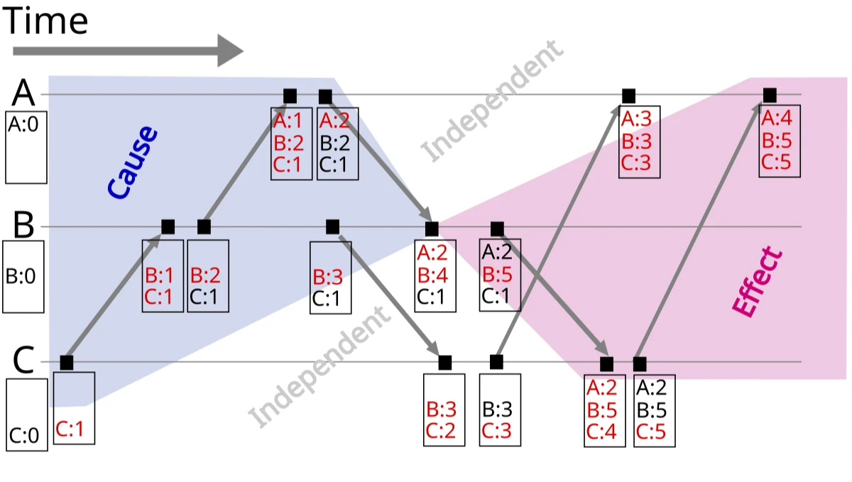
Vector Clocks: A Better Solution:
Vector clocks track causality between different versions of data:
Vector clocks tracking causality between events in a distributed system
Source: Wikipedia, "Vector clock" (https://en.wikipedia.org/wiki/Vector_clock)
Each node maintains a counter for every node in the system:
- When a node updates data, it increments its own counter
- When a node receives data from another node, it updates its vector clock
- Two vector clocks can be compared to determine if one event happened before another
Comparing Vector Clocks:
Looking at the image above, we can determine causality relationships:
- Causally Related: When all values in one vector clock are equal to or greater than another, and at least one value is strictly greater, there is a causal relationship. For example, vector clock [3,0,0] happens after [2,0,0] because all elements are greater than or equal to the elements in [3,0,0]
- Concurrent Events: When neither vector clock's values are all greater than or equal to the other, the events are concurrent. For example, [2,0,0] and [0,1,0] are concurrent because neither descends from the other.
Examples:
- [4,4,1] causally follows [3,0,0] because all elements in [4,4,1] are greater than or equal to the elements in [3,0,0]
- [2,3,1] and [2,0,0] are causally related because all elements in [2,3,1] are greater than or equal to [2,0,0]
- [2,2,0] and [2,4,1] are concurrent because [2,2,0] has elements not greater than [2,4,1] and vice versa
This comparison allows distributed systems to determine whether events have a happened-before relationship or occurred concurrently, which is crucial for conflict resolution.
Resolving Concurrent Conflicts with Vector Clocks:
Vector clocks help detect concurrent updates, but application-specific logic is needed to resolve conflicts. Consider a shopping cart scenario:
Example: Shopping Cart Operations
Starting state: Empty cart with vector clock [0,0,0]
Concurrent operations:
- Device A: Add Book → Vector clock [1,0,0]
- Device B: Add Headphones → Vector clock [0,1,0]
Conflict resolution: Merge both additions
- Result:
{Book: 1, Headphones: 1}
with vector clock [1,1,0]
When conflicting operations include removals, resolution becomes more complex:
Tombstones for Deletions:
In distributed systems, items aren't immediately deleted but marked with a "tombstone" indicating they were deleted:
Example:
- Starting cart:
{Book: 1, Headphones: 1}with vector clock [1,1,0] - Device B removes Book → Creates a tombstone, not just removing it
- Resulting data:
{Headphones: 1, Book: TOMBSTONE}with vector clock [1,2,0]
Tombstones ensure that deletions propagate correctly through the system. If another replica later tries to re-add the deleted item due to asynchronous replication, the tombstone indicates that the item was intentionally deleted and should remain so. Tombstones are typically garbage-collected after all replicas have acknowledged the deletion.
Sloppy Quorums and Hinted Handoff
In a distributed system, strict quorum requirements may not be possible during network partitions or node failures.
Sloppy Quorums:
- Allow writes and reads to proceed even if the "proper" nodes are unavailable
- Accept writes on behalf of unavailable nodes (temporary stewardship)
- Increases availability at the cost of consistency guarantees
Hinted Handoff:
- Nodes that accept writes on behalf of unavailable nodes store "hints"
- When the proper node becomes available again, the hints are delivered
- Ensures eventual consistency even after prolonged outages
Leader-Based Replication vs Leaderless Replication
| Aspect | Leader-Based Replication | Leaderless Replication |
|---|---|---|
| Availability | • Leader failure requires failover | • No single point of failure |
| Consistency | • Simpler consistency model | • Requires conflict resolution strategies |
| Latency | • Writes must go to leader | • Clients can write to closest node |
| Implementation | • Simpler implementation | • More complex conflict resolution |
| Use Cases | • Traditional RDBMS (MySQL, PostgreSQL) | • Distributed NoSQL databases (Cassandra, Riak) |
Conclusion
This article has explored the core concepts that power modern database systems:
Storage and Data Structures
- B-Trees and B+ Trees form the backbone of traditional relational databases, optimizing for read performance and range queries
- LSM Trees revolutionize write-heavy workloads by using in-memory buffers and sequential disk writes
- Both approaches make fundamental trade-offs in terms of read vs. write performance
Memory and Reliability
- Buffer pools bridge the gap between slow disk storage and fast memory access
- Write-ahead logging (WAL) ensures durability and atomicity even during system failures
Transaction Processing
- Isolation levels (Read Uncommitted to Serializable) balance performance against consistency guarantees
- Concurrency control techniques prevent anomalies like dirty reads, lost updates, and write skew
Distributed Database Architectures
- Partitioning schemes like consistent hashing distribute data across multiple nodes for horizontal scaling
- Replication approaches (leader-based, multi-leader, leaderless) provide fault tolerance with different consistency models
- Vector clocks track causality in distributed systems, enabling conflict detection and resolution
- Techniques like quorum consensus, read repair, and tombstones ensure eventual consistency in the face of network partitions
These fundamental concepts continue to evolve as databases adapt to new requirements for scale, availability, and performance. The right database for your application will depend on your specific workload characteristics and consistency requirements.